Chapter 25 Categorical data
Much of the time in biology, we are dealing with whole objects (plants, animals, cells, eggs, islands, etc.) or discrete events (attacks, matings, nesting attempts, etc.). We are often interested in making measurements of numeric variables (length, weight, number, etc.) and then either comparing means from samples (e.g. mean leaf size of plants from two habitat types) or investigating the association between different measurements (e.g. mean leaf size and herbivore damage).
However, we sometimes find a situation where the ‘measurement’ we are interested in is not a quantitative measure but is categorical. Categorical data are things like sex, colour or species. Such variables cannot be treated in the same way as numeric variables. Although we can ‘measure’ each object (e.g. record if an animal is male or female), we can’t calculate numeric quantities such as the ‘mean colour morph’, ‘mean species’ or ‘median sex’ of animals in a sample. Instead, we work with the observed frequencies, in the form of counts, of different categories, or combinations of categories.
25.1 A new kind of distribution
There are quite a few options for dealing with categorical data22. We’re just going to look at one option in this book: \(\chi^2\) tests. This is pronounced, and sometimes written, ‘chi-square’. The ‘ch’ is a hard ‘ch’, as in ‘character’. They aren’t necessarily the best tool for every problem, but \(\chi^2\) tests are widely used in biology, so they are a good place to start.
The material in this chapter is provided for readers who like to have a sense of how statistics works. Don’t worry too much if it seems confusing—you don’t have to understand it to use the tests we’ll cover in the next two chapters. In any case, this chapter is very short.
The \(\chi^2\) tests that we’re going to study borrow their name from a particular theoretical distribution, called… the \(\chi^2\) distribution. We won’t study this in much detail. However, just as with the normal distribution and the t-distribution, it can be helpful to know a bit about it:
- The \(\chi^2\) distribution pops up a lot in statistics. In contrast to the normal distribution, it isn’t often used to model the distribution of data. Instead, the \(\chi^2\) distribution is usually associated with a test statistic of some kind.
- The standard \(\chi^2\) distribution is completely defined by only one parameter, called the degrees of freedom. This is closely related to the degrees of freedom idea introduced in the chapters on t-tests.
- The \(\chi^2\) distribution is appropriate for positive-valued numeric variables. Negative values aren’t allowed. This is because the distribution arises whenever we take one or more normally distributed variables, square these, and then add them up.
Let’s take a look at the \(\chi^2\) distribution with one degree of freedom:
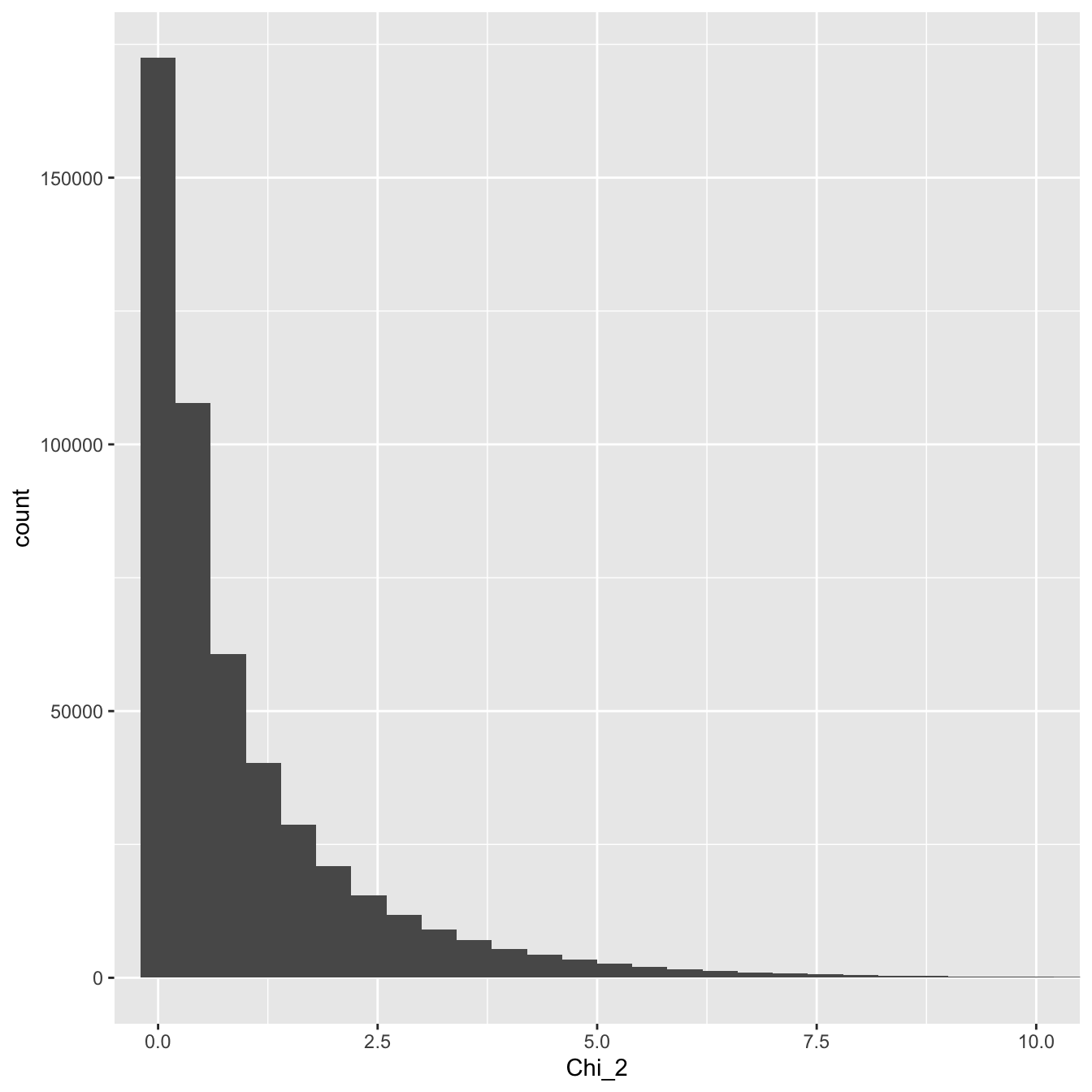
Figure 25.1: Distribution of a large sample of chi-square distributed variable with one degree of freedom
As we just noted, only positive values occur and most of these values lie between about 0 and 10. We can also see that the distribution is asymmetric. It is skewed to the right.
So why is any of this useful?
Let’s look at the plant morph example again. Imagine taking repeated samples from a population when the purple morph frequency is 25% . If we take 1000 plants each time and the true frequency is 25%, we expect to sample 250 purple plants on average. We’ll call this number the ‘expected value’. We won’t actually end up with 250 plants in each sample because of sampling error. We’ll call this latter number the ‘observed value’.
So far we’re not doing anything we haven’t seen before. We’re just discussing what happens under repeated sampling from a population. Here’s the new bit… Imagine that every time we sample the 1000 plants, we calculate the following quantity:
\[2*\frac{(O-E)^{2}}{E}\]
…where \(O\) is the observed value and \(E\) is the expected value defined above. What does its distribution look like? We can find out by simulating the scenario in R and plotting the results:
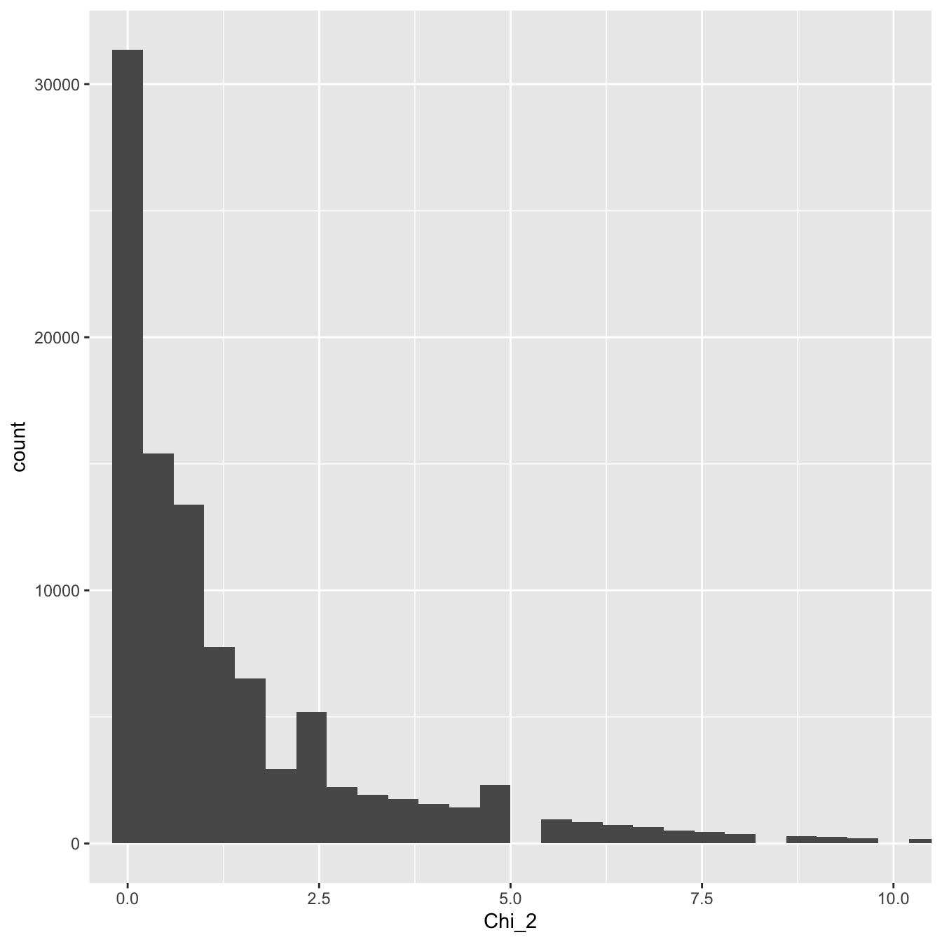
Figure 25.2: Distribution of the test statistic
That looks a lot like the theoretical \(\chi^2\) distribution we plotted above. It turns out that observed frequencies (‘counts’) that have been standardised with respect to their expected values—via the \(\frac{(O-E)^{2}}{E}\) statistic—have a \(\chi^2\) sampling distribution (at least approximately). This result is the basis for using the \(\chi^2\) distribution in various statistical tests involving categorical variables and frequencies or counts.
25.2 Types of test
We’re going to learn about two different types of \(\chi^2\) test. Although the two tests work on the same general principle, it is still important to distinguish between them according to where they are used.
25.2.1 \(\chi^{2}\) goodness of fit test
A goodness-of-fit test is applicable when we have a single categorical variable and some hypothesis from which we can predict the expected proportions of observations falling in each category.
For example, we might want to know if there is any evidence for sex-related bias in the decision to study biology at Sheffield. We could tackle this question by recording the numbers of males and females in a cohort. This would produce a sample containing one nominal variable (Sex) with only two categories (Male and Female). Based on information about human populations, we know that the sex ratio among 18-year-olds is fairly close to 1:123. We can thus compare the goodness of fit of the number of males and females in a sample of students with the expected value predicted by the 1:1 ratio.
If we had a total of 164 students, we might get this sort of table:
| Male | Female | |
|---|---|---|
| Observed | 74 | 90 |
With a 1:1 sex ratio, if there is no sex bias in the decision to study biology, we would expect 82 of each sex. It looks as though there might be some discrepancy between the expected values and those actually found. However, this could be entirely consistent with sampling variation. The \(\chi^{2}\) goodness of fit test allows us to test how likely it is that such a discrepancy has arisen through sampling variation.
25.2.2 \(\chi^{2}\) contingency table test
A contingency table test is applicable when each object is classified according to more than one categorical variable. Contingency table tests are used to test whether there is an association between the categories of those variables.
Consider biology students again. We might be interested in whether eye colour was in any way related to sex. It would be simple to record eye colour (e.g. brown vs blue) along with the sex of each student in a sample. Now we would end up with a table that had two classifications:
| Blue eyes | Brown eyes | |
|---|---|---|
| Male | 44 | 20 |
| Female | 58 | 42 |
Now it is possible to compare the proportions of brown and blue eyes among males and females… The total number of males and females are 64 and 100, respectively. The proportion of males with brown eyes is 20/64 = 0.31, and that for females 42/100 = 0.42. It appears that brown eyes are somewhat less prevalent among males. A contingency table test will tell us if the difference in eye colour frequencies is likely to have arisen through sampling variation.
Notice that we are not interested in judging whether the proportion of males, or the proportion of blue-eyed students, are different from some expectation. That’s the job of a goodness of fit test. We want to know if there is an association between eye colour and sex. That’s the job of a contingency table test.
25.2.3 The assumptions and requirements of \(\chi^{2}\) tests
Contingency tables and goodness-of-fit tests are not fundamentally different from one another in terms of their assumptions. The difference between the two types lies in the type of hypothesis evaluated. When we carry out a goodness-of-fit test, we have to supply the expected values. In contrast, the calculation of expected values is embedded in the formula used to carry out a contingency table test. That will make more sense once we’ve seen the two tests in action.
\(\chi^{2}\) tests are sometimes thought of as non-parametric tests because they do not assume any particular form for the distribution of the data. In fact, as with any statistical test, there are some assumptions in play, but these are relatively mild:
- The data are independent counts of objects or events which can be classified into mutually exclusive categories.
- The expected counts are not very low. The general rule of thumb is that the expected values should be greater than 5.
The most important thing to remember about \(\chi^{2}\) tests is that they must always be carried out on the actual counts. Although the \(\chi^{2}\) is telling us how the proportions of objects in categories vary, the analysis should never be carried out on the percentages or proportions, only on the original count data, nor can a \(\chi^{2}\) test be used with means.