Chapter 18 Paired-sample t-test
In the previous chapter, we learned how blocking is a valuable technique for dealing with confounding effects. However, we didn’t discuss how we would analyse such data. If we’ve used a block design, we can’t just throw our data at something like a t-test or a standard one-way ANOVA. Remember, one of the assumptions of these tests is the independence of the experimental units, yet a blocked design creates a situation where some units are not independent. In this chapter and the next, we’ll consider versions of the t-test and ANOVA that can be used to analyse such non-independent data.
18.1 When do we use a paired-sample t-test?
There are situations in which data may naturally form pairs of non-independent observations: the first value in sample A is linked to the first value in sample B, the second value in sample A is linked with the second value in sample B, and so on. This is known as a paired-sample data. A common example of paired-sample data is when we have a group of organisms, and we record some measurements from each organism before and after an experimental treatment. For example, if we were studying heart rate in relation to position (sitting vs standing), we might measure the heart rate of several people in both positions. In this case, the heart rate of a particular person when sitting is paired with the heart rate of the same person when standing.
An experimental design that sets out to produce paired data is known as a paired-sample design. More often than not, paired-sample data arise as a consequence of such deliberate decisions. Why? In biology, we often have the problem that there is a great deal of variation between the units we’re studying (individual organisms, tissue samples, etc). There may be so much among-unit variation that the effect of any difference among the situations we’re interested in is obscured. Using a paired-sample design gives us a way to control for the among-unit variation and increase the power of our statistical tests. However, we should not use a two-sample t-test when our data have this kind of structure. Let’s find out why.
18.2 Why do we use a paired-sample design?
Consider the following. A drug company wishes to test two drugs for their effectiveness in treating a rare illness in which glycolipids are poorly metabolised. An effective drug is one that lowers glycolipid concentrations in patients. The company can only find 8 patients willing to cooperate in the early trials of the two drugs. What’s more, the 8 patients vary in their age, sex, body weight, severity of symptoms and other health problems.
One way to conduct an experiment that evaluates the effect of the new drug is to randomly assign the 8 patients to one or other drug and monitor their performance. However, this kind of design is very unlikely to detect a statistically significant difference between the treatments. This is because it provides very little replication, yet can we expect considerable variability from one person to another in glycolipid levels before any treatment is applied. This variability would lead to a large standard error in the difference between means.
A solution to this problem is to treat each patient with both drugs in turn and record the glycolipid concentrations in the blood after taking each drug. One arrangement would be for four patients to start with drug A and four with drug B, and then after a suitable break from the treatments, they could be swapped over onto the other drug. This would give us eight replicate observations on the effectiveness of each drug, and we can determine, for each patient, which drug is more effective.15
The experimental design, and one hypothetical outcome, is represented in the diagram below…
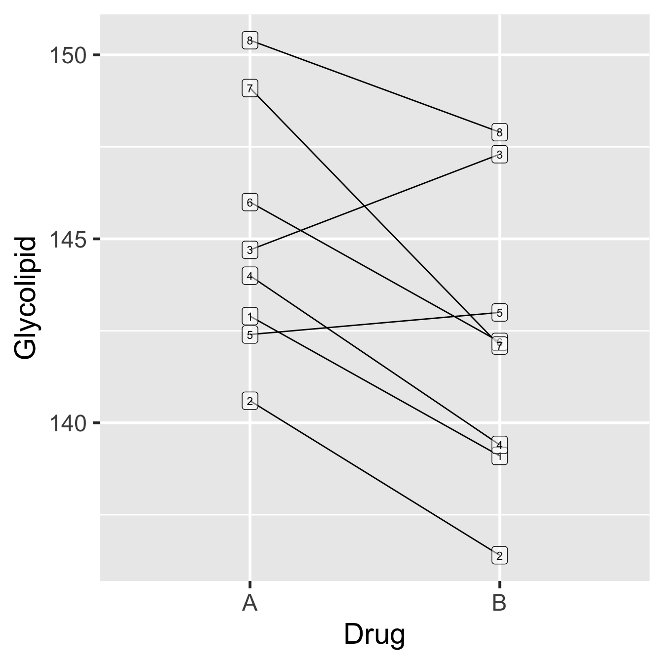
Figure 18.1: Data from glycolipid study, showing paired design. Each patient is denoted by a unique number.
Each patient is represented by a unique number (1-8). The order of the drugs in the plot does not matter—it doesn’t mean that Drug A was tested before Drug B just because Drug A appears first. Notice that there is a lot of variability in these data, both in the glycolipid levels of each patient and in the amount by which the drugs differ in their effects (e.g. the drugs have roughly equal effects for patient 5, while drug B appears to be more effective for patient 2). What can also be inferred from this pattern is that although the glycolipid levels vary a good deal between patients, Drug B seems to reduce glycolipid levels more than Drug A.
The advantage to using a paired-sample design in this case is clear if we look at the results we might have obtained on the same patients, but where they have been divided into two groups of four, giving one group Drug A and one group Drug B:
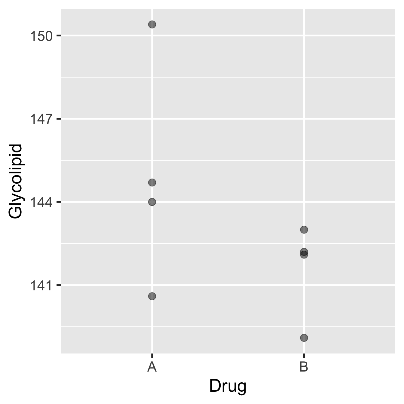
Figure 18.2: Data from glycolipid study, ignoring paired design.
The patients and their glycolipid levels are identical to those in the previous diagram, but now, patients 2, 3, 4 and 8 (selected at random) were given Drug A, while only patients 1, 5, 6, and 7 were given Drug B. The means of the two groups are different, with Drug B performing better, but the associated standard error are also large relative to this difference. A two-sample t-test would undoubtedly fail to identify a significant difference between the two drugs.
So, it would be quite possible to end up with two groups where there was no apparent difference in the mean glycolipid levels between the two drug treatments even though Drug B seems to be more effective in the majority of patients. The pairing allows us to factor out (i.e. remove) the variation among individuals and concentrate on the differences between the two treatments. This works by focussing on the differences occurring within individuals. The result is a much more sensitive evaluation of the effect we’re interested in.
The next question is, how do we go about analysing paired data in a way that properly accounts for the structure in the data?
18.3 How do you carry out a t-test on paired samples?
It should be clear why a paired-sample design might be useful, but how do we construct the right test? The ‘trick’ is to work directly with the differences between pairs of values. In the case of the glycolipid levels illustrated in the first diagram, we noted that there was a greater decrease of glycolipids in 75% of patients using Drug B compared with Drug A.
If we calculate the actual differences (i.e. subtracted the value for Drug A from the value for Drug B) for each patient, we might see something like: -3.9, -4.1, 2.5, -4.7, 0.5, -3.7, -6.9, -2.4. Notice that there are only two positive values in this sample of differences, one of which is close to 0. The mean difference is -2.8, i.e. on average, glycolipid levels are lower with Drug B. Another way of stating this observation is that within subjects (patients), the mean difference between drug B and drug A is negative. A paired-sample design focusses on the within-subject (or more generally, within-item) change.
On the other hand, if the two drugs had had similar effects, what would we expect to see? We would expect no consistent difference in glycolipid levels between the Drug A and Drug B treatments. Glycolipid levels are unlikely to remain exactly the same over time. Still, there shouldn’t be any pattern to these changes with respect to the drug treatment: some patients will show increases, some decreases, and some no change at all. The mean of the differences, in this case, should be somewhere around zero (though sampling variation will ensure it isn’t exactly equal to zero).
So, to carry out a t-test on paired-sample data, we have to: 1) find the mean of the difference of all the pairs and 2) evaluate whether this is significantly different from zero. We already know how to do this! This is just an application of the one-sample t-test, where the expected value (i.e. the null hypothesis) is 0. The thing to realise is that although we started out with two sets of values, what matters is the sample of differences between pairs and the population we’re interested in a ‘population of differences’.
When used to analyse paired data in this way, the test is referred to as a paired-sample t-test. This is not wrong, but it is important to remember that a paired-sample t-test is just a one-sample t-test applied to the sample of differences between pairs of associated observations. A paired-sample t-test isn’t a new kind of test. Instead, it is a one-sample t-test applied to a particular kind of situation.
18.3.1 Assumptions of the paired-sample t-test
The assumptions of a paired-sample t-test are no different from the one-sample t-test. After all, they boil down to the same test! We just have to be aware of the target sample. The key point to keep in mind is that the sample of differences is important, not the original data. There is no requirement for the original data to be drawn from a normal distribution because the normality assumption applies to the differences. This is very useful because even where the original data seem to be drawn from a non-normal distribution, the differences between pairs can often be acceptably normal. The differences need to be measured on an interval or ratio scale, but this is guaranteed if the original data are on one of these scales.
18.4 Carrying out a paired-sample t-test in R
R offers the option of a paired-sample t-test to save us the effort of calculating differences. It does this for us and then carries out a one-sample test on those differences. We’ll look at how to do it the ‘old fashioned’ way first—calculating the differences ourselves and running a one-sample test—before using the short-cut method provided by R. We’ll do this using the glycolipid drug example.
The data live in the ‘GLYCOLIPID.CSV’ file. The code below assumes those data have been read into a tibble called glycolipid. Set that up if you plan to work along.
We start by looking at the data:
## Rows: 16
## Columns: 4
## $ Patient    <dbl> 1, 2, 3, 4, 5, 6, 7, 8, 1, 2, 3, 4, 5, 6, 7, 8
## $ Sex        <chr> "Male", "Female", "Male", "Female", "Female", "Male", "Fema…
## $ Drug       <chr> "A", "A", "A", "A", "A", "A", "A", "A", "B", "B", "B", "B",…
## $ Glycolipid <dbl> 142.9, 140.6, 144.7, 144.0, 142.4, 146.0, 149.1, 150.4, 139…
There are four variables in this data set: Patient indexes the patient identity, Sex is the sex of the patient (we don’t need this), Drug denotes the drug treatment, and Glycolipid is the glycolipid level.
Next, we need to calculate the differences between each pair. We can do this with the dplyr functions group_by and summarise:
What we did was group the data by the values of Patient, and then used a function called diff to calculate the difference between the two Glycolipid concentrations within each patient. We stored the result of this calculation in a new data frame called glycolipid_diffs. This is the data we’ll use to carry out the paired-sample t-test:
## # A tibble: 8 × 2
##   Patient Difference
##     <dbl>      <dbl>
## 1       1     -3.80
## 2       2     -4.20
## 3       3      2.60
## 4       4     -4.60
## 5       5      0.600
## 6       6     -3.80
## 7       7     -7
## 8       8     -2.5
We should check that the differences could plausibly have been drawn from a normal distribution, though keep in mind that the normality assumption is hard to assess with only 8 observations:
## Bin width defaults to 1/30 of the range of the data. Pick better
## value with `binwidth`.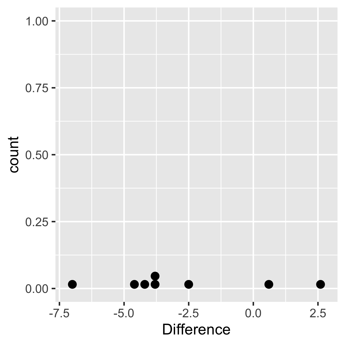
Figure 18.3: Within-individual differences from glycolipid study
Hmm… there really isn’t a lot of data to work with here but there’s nothing in that plot that screams ‘non-normal’, which means the assumptions have been met as best they can be. Let’s proceed to carry out a one-sample t-test on the calculated differences. This is easy to do in R:
##
##  One Sample t-test
##
## data:  glycolipid_diffs$Difference
## t = -2.6209, df = 7, p-value = 0.03436
## alternative hypothesis: true mean is not equal to 0
## 95 percent confidence interval:
##  -5.397549 -0.277451
## sample estimates:
## mean of x
##   -2.8375
We don’t have to set the data argument to carry out a one-sample t-test on the differences. We just passed along the numeric vector of differences extracted from glycolipid_diffs (using the $ operator). What happened to the mu argument used to set up the null hypothesis? Remember, the null hypothesis is that the population mean is zero. R assumes that this is 0 if we don’t supply it, so no need to set it here.
The output is quite familiar… The first line reminds us what kind of test we did, and the second line reminds us what data we used to carry out the test. The third line is the important one: t = -2.6209, df = 7, *p*-value = 0.03436. This gives the t-statistic, the degrees of freedom, and the all-important p-value associated with the test. The p-value tells us that the mean within-individual difference is significant at the p < 0.05 level.
We need to express these results in a clear sentence incorporating the relevant statistical information:
Individual patients had significantly lower serum glycolipid concentrations when treated with Drug B than when treated with Drug A (t = 2.62, d.f. = 7, p < 0.05).
There are a couple of things to point out in interpreting the result of such a test:
The sample of differences was used in the test, not the sample of paired observations. This means the degrees of freedom for a paired-sample t test are one less than the number of differences (= number of pairs); not one, or two, less than the total number of observations.
Since we used a paired-sample design our conclusion stresses the fact that the use of the Drug B results in a lower glycolipid level in individual patients. It doesn’t say that the use of Drug B resulted in lower glycolipid concentrations for everyone given Drug B than for anyone given Drug A.
18.4.1 Using the Pair() interface for paired t-tests
Since version 4.5, R provides a clearer and more explicit way to run paired-sample t-tests, using the Pair() interface. The logic is the same as before — we want to compare two measurements (Drug A vs. Drug B) taken from the same participants — but now we’ll make that pairing explicit in the data we give to t.test().
Our original glycolipid data are in long format—each row represents a single measurement for a patient, with one column for the drug name and another for the glycolipid level:
## # A tibble: 16 × 4
##    Patient Sex    Drug  Glycolipid
##      <dbl> <chr>  <chr>      <dbl>
##  1       1 Male   A           143.
##  2       2 Female A           141.
##  3       3 Male   A           145.
##  4       4 Female A           144
##  5       5 Female A           142.
##  6       6 Male   A           146
##  7       7 Female A           149.
##  8       8 Female A           150.
##  9       1 Male   B           139.
## 10       2 Female B           136.
## 11       3 Male   B           147.
## 12       4 Female B           139.
## 13       5 Female B           143
## 14       6 Male   B           142.
## 15       7 Female B           142.
## 16       8 Female B           148.
To use the new Pair() interface, we first need to reshape the data into wide format, where each patient’s two measurements occupy a single row — one column for Drug A and one for Drug B.
We can do this with the pivot_wider() function from the tidyverse tidyr package. We have to load and attach the package to use it:
Then we select the three variable we want to keep and use pivot_wider to reshape the data:
# convert to wide format data
glycolipid_wide <- glycolipid %>%
  select(Patient, Drug, Glycolipid) %>%
  pivot_wider(
    names_from  = Drug,
    values_from = Glycolipid
  )
The wide format glycolipid_wide version of the data look like this:
## # A tibble: 8 × 3
##   Patient     A     B
##     <dbl> <dbl> <dbl>
## 1       1  143.  139.
## 2       2  141.  136.
## 3       3  145.  147.
## 4       4  144   139.
## 5       5  142.  143
## 6       6  146   142.
## 7       7  149.  142.
## 8       8  150.  148.
How does pivot_wider work here?
names_from = Drugtells R to take the values in theDrugcolumn (i.e."A"and"B") and turn them into new column names.values_from = Glycolipidtells R to fill those new columns with the corresponding glycolipid measurements.- Because we also keep
Patient, each patient now appears once in the data, with both of their measurements side by side.
Now that our data are in the right shape, we can run the paired t-test using the Pair() syntax:
##
##  Paired t-test
##
## data:  Pair(B, A)
## t = -2.6209, df = 7, p-value = 0.03436
## alternative hypothesis: true mean difference is not equal to 0
## 95 percent confidence interval:
##  -5.397549 -0.277451
## sample estimates:
## mean difference
##         -2.8375
This performs the same paired-sample t-test as before, but the code now makes it very clear which two columns form the pair. R still does the differencing for us behind the scenes, so we don’t need to create a separate data frame of differences. The output should be exactly the same as above so we’ll not discuss it again.
This kind of experimental design is called a cross-over study. It can be problematic if, for example, “carry-over” effects occur, e.g., the effect of one drug is altered when the other drug has previously been administered. We won’t worry about these problems here though.↩︎